BLOGS WEBSITE

Introduction

This is the last (for now) post in a series about about i-arrows, which are a way I have created of visualising the complex points on graphs in the real plane. As I’ve done for every other post since the first one, I will repeat the description here.

Every point with complex coordinates is represented as an arrow (which I call an “i-arrow”) from one place to another on top of the Cartesian plane.

  • Real points are dots on the Cartesian plane, the same as they have always been.
  • The complex point (p+si,q+ti) is represented as an i-arrow, which is an arrow based at the point (p,q) and extends along the vector (s,t) to have its arrowhead at the point (p+s,q+t).

In the picture below, there are three examples of i-arrows.

  • The complex point (1+4i,2+i) has been drawn as an i-arrow. Its base is at the point (1,2) and its arrowhead is at the point (1+4,2+1)=(5,2).
  • The complex point (7,2i) has been drawn as an i-arrow. Its base is at the point (7,0) and its arrowhead is at the point (7,0+2)=(7,2).
  • The complex point (12-2i,3) has been drawn as an i-arrow. Its base is at the point (12,3) and its arrowhead is at the point (12-2,3)=(10,3).

In the previous blog post, I talked about the complex points on a real circle, with an equation like (x-g)²+(y-h)²=R for a positive number R. In this blog post, I’ll talk about the complex points on an unreal circle.

Circles with negative area

The equation x²+y² = R for positive number R represents a circle in the sense that the collection of points (x,y) with real coordinates that satisfy the equation are indeed a circle. The area of that circle will be πR and its radius is √R.

The equation x²+y² = -R for positive number R represents nothing at all. There are no real numbers x and y that satisfy this equation, because when you square real numbers, you can’t get a negative result. And that’s that.

Except it’s not. That first equation equation x²+y² = R has a large number of points (x,y) with complex coordinates that satisfy it, and when you draw those points as i-arrows, they have a beautiful and surprisingly simple structure. There are definitely going to be points with complex coordinates that satisfy x²+y² = -R, and it would be completely unsurprising if they also had a beautiful and simple structure.

If the circle with equation x²+y² = R  has area πR and radius is √R, then it seems fair to say that the area of the circle with equation x²+y² = -R is -πR and its radius is √(-R) = √R i. So I am going to say that this circle has negative area and imaginary radius.

Ever since I found a way of thinking about where complex points are, I’ve wanted to investigate what circles with negative area look like. Now I finally can do it properly, with i-arrows.

Complex points on a circle with negative area: the i-arrows at each point

Just like I did for real circles, I’ll start by substituting in a general complex point and see what happens.

Consider the equation of a circle with negative area, x²+y² = -R, for positive real number R. Let (p+si,q+ti) be a complex point, for real numbers, p, q, s, t, and suppose (p+si,q+ti) satisfies the equation x²+y² = -R.

(p+si)²+(q+ti)² = -R
p² + 2psi – s² + q² + 2qti – t² = -R
p² + q² – s² – t² + (2ps+2qt)i = -R

Equate real and imaginary parts.

Imaginary:
2ps + 2qt = 0
ps + qt = 0
(p,q) • (s,t) =0
This tells me that the vector (s,t) is perpendicular to the vector (p,q), which goes from the origin to the point (p,q). This is the same as what happened for a real circle.

Real:
p² + q² – s² – t² = -R
p² + q² +R =  s² + t²
s² +  t² = p² + q² + R
√(s² +  t²) = √(p² + q² + R)
||(s,t)|| = √(p² + q² + R)
Again this is almost the same as what happened for a real circle. I have the possible directions from the imaginary part, and a formula for the length from the real part, which is enough to locate the i-arrow. But the geometrical interpretation is just a little different.

It is still true that √(p² + q²) is the length of the journey from the origin to (p,q) and that this length, √R and ||(s,t)|| are related by a Pythagoras-theorem-like expression. But this time, the different parts are playing different roles. Now, ||(s,t)|| is the hypotenuse of the triangle, and √R and √(p² + q²) are the short sides.


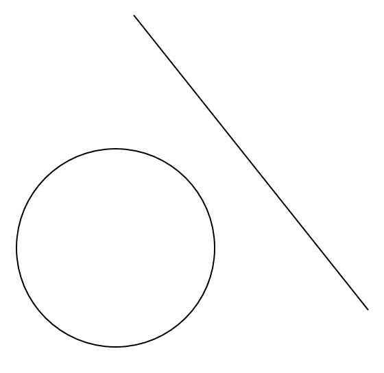
Last time, the right-angle told me there was a tangent to the circle, but this time that’s not going to happen. That right angle has to be at the origin, which is the centre of the circle, so it’s just not going to work. So my hope for a nice geometrical construction fades. After playing around, this is the best I can do.

To find the complex points on the circle of negative area x²+y² = -R whose i-arrows are based at P=(p,q):

  1. Draw the line from the origin to P.
  2. Draw a circle of radius √R centred at the origin.
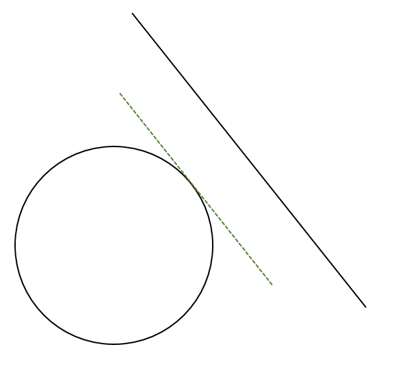
  3. Draw a diameter of this circle perpendicular to the line from the origin to P and mark where it meets the circle.
  4. Draw a circle centred at P passing through the two points on that diameter just marked.
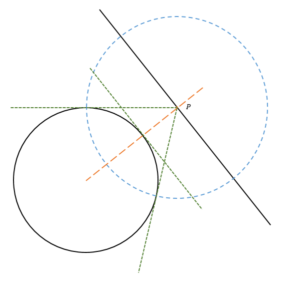
  5. Draw a line through P perpendicular to the line from the origin to P and mark where it meets the circle just drawn.
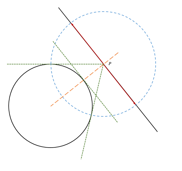
  6. The two points just marked are the arrowheads of the i-arrows based at P.

Actually a fairly simple construction now I’ve seen the picture! I note that the construction will work no matter whether P is inside, outside or on the edge of that dotted-line circle of radius √R, so for any point P there will always be complex points whose i-arrows are based there.

This bears out in the algebra, since (p² + q² + R) is always going to be greater than zero — in fact it will always be greater than or equal to R — there will always be a result for √(p² + q² + R) and so always a solution for the length of (s,t).

There is one special case I notice though: when (p,q) is the origin. In that case the length of (s,t) will still have an answer, which will be √R. But also (p,q) • (s,t) =0 for every possible vector (s,t). So actually every vector based at the origin of length √R is an i-arrow on this circle! That is, given any point P, there are two i-arrows on the unreal circle based there, unless P is the origin, in which case there are infinitely many i-arrows on the unreal circle based there, and their arrowheads form a circle of radius √R. I think this is so cool! The imaginary circle really does contain an imaginary circle in its complex points.

I guess the last thing to do is to calculate the coordinates of the arrowheads for the i-arrows at a specific point (p,q). This ought to be very similar to what happened for a real circle.

The vector (s,t) is perpendicular to the vector (p,q), so it’s some multiple of (q,-p).
Let’s say (s,t)=m(q,-p).
The length of (s,t) now has two ways to figure it out.

||(s,t)|| = ||m(q,-p)||
= |m| ||(q,-p)||
= |m| √(p² + q²)
and
||(s,t)|| = √(p² + q² + R)

So
|m| √(p² + q²) = √(p² + q² + R)
|m| = √(p² + q² + R) / √(p² + q²)
= √[1 + R/(p² + q²)]

Therefore
(s,t) = ±√[1 + R/(p² + q²)] (q,-p)

And so the arrowheads of the i-arrows based at (p,q) are at
(p+q√[1 + R/(p² + q²)], q-p√[1 + R/(p² + q²)])
and
(p-q√[1 + R/(p² + q²)], q+p√[1 + R/(p² + q²)]).

Yes, this is exactly the same as what happened for a real circle. Indeed, if I have the equation x² + y²=R and allow the number R to be negative, I get this for the locations of the arrowheads of the i-arrows based at (p,q) either way:
(p+q√[1 – R/(p² + q²)], q-p√[1 – R/(p² + q²)])
and
(p-q√[1 – R/(p² + q²)], q+p√[1 – R/(p² + q²)]).

How nice. What this means is it’s actually very easy to set up a GeoGebra activity that covers both real and unreal circles. This is precisely why I have been doing the equations as x² + y²=R as opposed to x² + y²=r², by the way. So that I could smoothly transition from real to unreal without a major change in the algebra. Well I hoped it would turn out that way, and I’m glad it did.

Collections of complex points on an unreal circle

And now I really can investigate the complex points on an unreal circle properly and look at collections of them all at once.

All the i-arrows at once

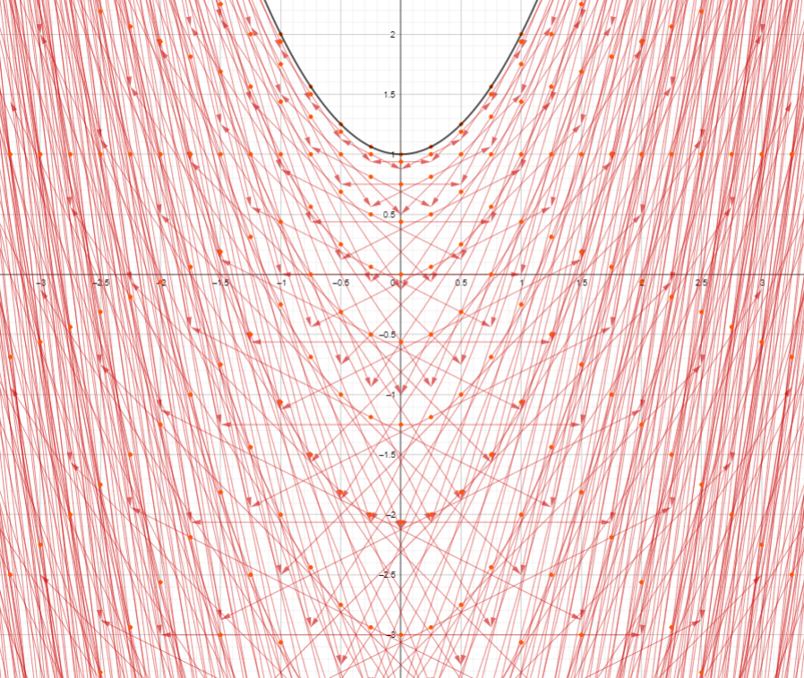
First, all the i-arrows for the complex points on the circle x²+y² = -4 of negative area based at the points on a grid with spacing 1/4. (You can play around with this for different values of R, including both positive and negative, as well as different grid spacings, using this GeoGebra activity.

As you can see, there are a lot more lines and arrowheads than there were for the real circle of the matching real radius, due to there being i-arrows based at every point, rather than only ones outside a circle. I think I can at see a space in the middle there that is less red. When I look closer it’s not just that there are fewer arrows there, but specifically fewer arrowheads. But there are almost too many arrows for me to see clearly. Let me try again with a wider grid spacing. This picture is the same but with a grid spacing of 1/2.

I can more easily distinguish that circle of i-arrows at the origin from the rest of the i-arrows, and it’s making me even more sure that there are no arrowheads inside that circle. Let me see if I can confirm that…

The arrowheads of the i-arrows based at the non-origin point (p,q) are given by
(p+q√[1 + R/(p² + q²)], q-p√[1 + R/(p² + q²)])
and
(p-q√[1 + R/(p² + q²)], q+p√[1 + R/(p² + q²)]).

Phew that’s complicated. What if I let m = √[1 + R/(p² + q²)] so that the arrowheads are at
(p+qm,q-pm) and (p-qm,q+pm).

These points will be outside the circle of radius R when their x and y coordinates satisfy x²+y²>R. Let me see what I get for that calculation for the first point.

x²+y²
= (p+qm)²+(q-pm)²
= p² + 2pqm + q²m² + q² – 2qpm + p²m²
= p² + q² + p²m² + q²m²
= p² + q² + (p² + q²)m²
= (p²+q²)(1+m²)

Note the same result would have happened if I had used the other point, because the -2pqm and +2qpm would have appeared in the other order but still had a sum of zero.

Now m = √[1 + R/(p² + q²)]
So m² = 1 + R/(p² + q²).

Therefore
x²+y²
= (p²+q²)(1+m²)
= (p²+q²)(1+1 + R/(p² + q²))
= (p²+q²)(2 + R/(p² + q²))
= 2(p²+q²)+R,
which is definitely greater than or equal to R.

I also notice that if this was a real circle with radius √R, then the arrowhead’s coordinates substituted into x²+y² would have produced 2(p²+q²)-R, which is also greater than or equal to R, since the only points with i-arrows are outside the circle where p²+q²>R. Very nice.

So for an unreal circle with equation x²+y² = -R (for positive R), the i-arrows for its complex points have arrowheads that are all outside the circle of radius √R, plus the circle of i-arrows at the origin, whose arrowheads are the whole of the circle of radius √R itself.

The i-arrows on a vertical line

You can play around with what the i-arrows based at points along a vertical line look like in this GeoGebra activity. It will allow you to change the value of R to be both positive and negative to compare how both real and unreal circles work.

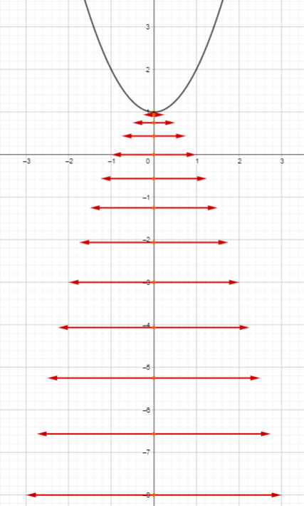
Here is GIF showing a selection of i-arrows on the unreal circle x²+y² = -4 based at points on a vertical line as the line moves back and forth. (The real circle with equation  x²+y² = 4 has been shown for reference.)

It’s a bit jerky, I’m sorry, but GeoGebra was working hard, and also I moved the slider manually because I wanted it to show the circle of i-arrows at the origin for a moment as I went past. I just love that it’s there at that one moment. Actually, what happens at that moment is pretty cool.

As well as the circle of i-arrows at the origin, the arrowheads for all the i-arrows seem to be forming a hyperbola, like they did for a real circle, but the other way around. That definitely deserves investigating, and it ought to look very similar to how it looked for a real circle.

The vectors that are the i-arrows at the point (p,q) are given by
±√[1 + R/(p² + q²)] (q,-p).

If p=0, these vectors are
±√[1 + R/q²] (q,0)
= ±√[q² + R] (1,0).
This confirms that all the i-arrows based along the y-axis are horizontal.

The arrowheads of the arrowheads of the i-arrows based at the point (p,q) are given by
(p,q)±√[1 + R/(p² + q²)] (q,-p).

If p=0, these points are
(0,q)±√[q² + R] (1,0)
= (±√[q² + R],q).

When you take the x-coordinates and y-coordinates and square them, you get this:
x²=q²+R
y²=q²
x²-y²=R
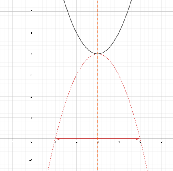
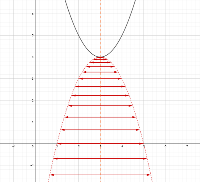
That is indeed the equation of a hyperbola with turning points at (√R,0) and (-√R,0).

Awesome. I am particularly loving how this unreal circle is highlighting the intimate relationship between a circle and a hyperbola.

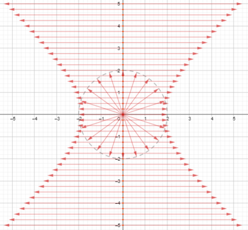
The i-arrows on the lines through the origin

This hyperobola of i-arrow arrowheads should appear not just for i-arrows based along the y-axis, but along any line through the origin, which means I can cover all the i-arrows on the unreal circle systematically by looking at the ones attached to a rotating line through the origin. Here is the GeoGebra activity that lets you do this for circles of both positive and negative area. And here is the GIF of the i-arrows for the complex points on the unreal circle x²+y² = -4 based at equally-spaced points along a rotating line.

The i-arrows based at points around a circle

Jim Simons on twitter suggested for a real circle to organise the i-arrows by how far their base is from the centre, and it really is a good idea. Here is the GeoGebra activity that will let you investigate this selection of i-arrows for both real and unreal circles. And here is a GIF showing the i-arrows on the negative unit circle with equation x²+y² = -1, organised by how far their base is from the centre.

I really love this GIF. I love how the i-arrows are longer and longer the further out from the centre they are based, but also I love how the circle of i-arrows at the origin seems perfectly natural now because that’s where the i-arrows based at points around a very small circle are converging towards.

Conclusion

I am very satisfied to have finally got a handle on what is happening with these circles of negative area. I love how the complex points on both the real and unreal circles have that hyperbola of arrowheads formed by the i-arrows based along a line through the circle’s centre. It’s just so simple and clean. Even more than this, I just love that circle of i-arrows based at the centre of an unreal circle. It’s just so very circley and simultaneously unreal, just like you would hope on an unreal circle. Just to draw all of this together, here is a GIF of the hyperbola of arrowheads for the i-arrows along a rotating line for circles x²+y² = R, with R ranging from -5 to 5.

I feel like this GIF really highlights the similarities and differences between the circles of positive and negative area. Also it’s just super cool. I could watch it all day long.

As an aside: one thing you can notice in the above GIF is the momentary transition between the positive and negative area circles. In that case, there is exactly one real point, which is the origin, and we’ve seen things like that before: in unreal lines. This actually does make sense, because x²+y² = 0 can be factorised into (y+ix)(y-ix)=0, which is the two lines y=ix and y=-ix. It seems like one more way to make sense of a line of unreal slope is to think about it as half of a circle (or possibly an ellipse?) with zero area. But that’s another story and shall be told at another time.

This GIF shows the i-arrows on the positive and negative unit circles x²+y² = 1 and x²+y² = -1, with each frame showing the i-arrows at points around a circle. I feel this one really highlights the similarities and differences between positive and negative area circles. Again, I could watch it all day long.

I’ve certainly had a great time using i-arrows to investigate the complex points on a variety of shapes. If you’ve been following along, or just now come to just a part of it, I hope you’ve had a good time too. But for now, it’s time to sign off. They’ll still be there waiting when I come back one day.

One last time, these are all the other posts in this blog series, if you want to find them.

Posted in Isn't maths cool? | Tagged
Leave a comment

Introduction

This is the second last (it was going to be the last, but it got too big so I made it a separate one) in a series of blog posts about i-arrows: a way I have created of visualising complex points on real graphs. The first blog post described how they work, and I repeat the description here.

Every point with complex coordinates is represented as an arrow (which I call an “i-arrow”) from one place to another on top of the Cartesian plane.

  • Real points are dots on the Cartesian plane, the same as they have always been.
  • The complex point (p+si,q+ti) is represented as an i-arrow, which is an arrow based at the point (p,q) and extends along the vector (s,t) to have its arrowhead at the point (p+s,q+t).

In the picture below, there are three examples of i-arrows.

  • The complex point (1+4i,2+i) has been drawn as an i-arrow. Its base is at the point (1,2) and its arrowhead is at the point (1+4,2+1)=(5,2).
  • The complex point (7,2i) has been drawn as an i-arrow. Its base is at the point (7,0) and its arrowhead is at the point (7,0+2)=(7,2).
  • The complex point (12-2i,3) has been drawn as an i-arrow. Its base is at the point (12,3) and its arrowhead is at the point (12-2,3)=(10,3).

In this blog post, I’ll work through using i-arrows to represent the complex points on real circles. I did real circles about two years ago using my older idea of i-planes, but the i-arrows are so much better and will allow me to visualise things and talk about things much more easily.

The complex points on a real circle: i-arrows based at each point

I will investigate the complex points on the real circle with equation x²+y² = R for positive number R. In the previous post, I investigated the complex points on a parabola using the fact it was the graph of a function. I was able to get GeoGebra to do calculations using the function and show me the results. Unfortunately, circles are not the graphs of functions, so I won’t be able to do that here. Yes I know the two halves of a circle are the graphs of separate functions, but they have square roots, which can be a bit weird with complex numbers, so it’s safer not to do that. I will have to try to find the complex points on the real circle by seeing what happens when I substitute in a general point. I have done all this before, but I am happy to do it again. It is going to be ever so slightly different this time.

Let (p,q) be a fixed real point, and suppose the complex point (p+si,q+ti), for some real s and t, satisfies the circle’s equation. So

(p+si)²+(q+ti)² = R
p² + 2psi – s² + q² + 2qti – t² = R
p² + q² – s² – t² + (2ps+2qt)i = R

Equate real and imaginary parts.

Real:
p² + q² – s² – t² = R
p² + q² – R =  s² + t²
s² +  t² = p² + q² – R

Imaginary:
2ps + 2qt = 0
ps + qt = 0

Looking at these two equations, they look like they’re telling me about the vector (s,t). I have been trying to avoid talking about the i-arrows as vectors, but this is what the equations seem to be telling me to do.

The imaginary equation can be rewritten as a dot product:
ps + qt = 0
(p,q) • (s,t) =0
And this tells me that the point (p,q) imagined as a vector is perpendicular to the vector (s,t).

The real equation can have its square root done:
s² +  t² = p² + q² – R
√(s² +  t²) = √(p² + q² – R)
||(s,t)|| = √(p² + q² – R)
And this tells me what the length of the vector (s,t) is.

So I know the possible directions and the length of the vector (s,t), which is enough information to actually draw the i-arrows. Nice!

Except there are some details to sort out…

First, that length for the vector (s,t) isn’t going to exist if p²+q²-R is a negative number. That is, if p²+q²<R, then there will be no i-arrows with base at the point (p,q). But p²+q²<R happens exactly when the point (p,q) is inside the circle. So there are no i-arrows based at points inside the circle. If p²+q²=R, then (s,t) will have length 0 and there is no i-arrow at all. But that’s ok, because (p,q) is then a point on the real circle anyway. Finally, if p²+q²>R, then √(p²+q²-R) definitely exists, so there are definitely vectors of that length, and we’ll get two of them: one in each direction perpendicular to (p,q).

So I now know there are two i-arrows based at every point outside the circle, and none based at any point inside the circle. I know they point perpendicularly to the journey from the origin to the point where they are based. And I have a formula for how long they are. Let me look closer at that formula.

The number √(p²+q²) is how far (p,q) is from the origin, and the number √R is the radius of the circle. That means that √(p²+q²-R) is the length of the other short side of a right-angled triangle with long side the length of (p,q) and short side the radius of the circle.

The vertical edge in the picture is a radius of the circle, and the hypotenuse is the line from the origin to the point (p,q). The horizontal edge is perpendicular to the radius, so it has to be a tangent to the circle. That means the correct distance is the length of the tangent from (p,q) to the circle!  Very cool.

I still haven’t actually found the i-arrow yet though. The top edge in that picture isn’t actually the i-arrow itself, it’s just the length of the i-arrow. The i-arrow has to be perpendicular to the line from the origin to (p,q), and the top edge of that triangle is not. I need to draw arrows of that length in the right directions. To make sure they’re the right length, I can draw a circle of that radius. Then I can draw the arrows perpendicular to the line to (p,q).

Interestingly, if I draw both tangents from (p,q) to the circle, then the line joining the places where they meet the circle will also be perpendicular to the line from the origin to (p,q). So instead of going perpendicular to the line from the origin to (p,q), I could go parallel to the line joining the two points of tangency. This is kind of pleasant, because points inside the circle have no tangents of the circle through them, which would explain why the construction doesn’t work there.

So here’s a geometrical process for finding the i-arrows based at a point (p,q) outside the circle:

  • Draw the tangents from (p,q) to the circle and mark the points of tangency.
  • Draw a circle with centre (p,q) through those points of tangency.
  • Draw the line through those points of tangency.
  • Draw a line parallel to this one through the point (p,q).
  • The intersections of this line just drawn with the circle just drawn are the two arrowheads of the i-arrows.

Of course, if I want GeoGebra to draw the points, it might be easier to actually figure out their coordinates…

The vector (s,t) is perpendicular to the vector (p,q), so it’s some multiple of (q,-p).
Let’s say (s,t)=m(q,-p).
The length of (s,t) now has two ways to figure it out.

||(s,t)|| = ||m(q,-p)||
= |m| ||(q,-p)||
= |m| √(p² + q²)
and
||(s,t)|| = √(p² + q² – R)

So
|m| √(p² + q²) = √(p² + q² – R)
|m| = √(p² + q² – R) / √(p² + q²)
= √[1 – R/(p² + q²)]

Therefore
(s,t) = ±√[1 – R/(p² + q²)] (q,-p)

And so the arrowheads of the i-arrows based at (p,q) are at
(p+q√[1 – R/(p² + q²)], q-p√[1 – R/(p² + q²)])
and
(p-q√[1 – R/(p² + q²)], q+p√[1 – R/(p² + q²)]).

Where a circle meets an external line

I was going to use the algebraic calculations above to investigate collections of i-arrows, but I have noticed that the geometrical construction I drew before could actually help me find the complex points where a line that doesn’t meet the circle in a real point, actually does meet the circle.The trick is to find the point where they are based, then do the above construction to find the arrowheads.

Here is the construction.

  1. Draw the circle and the line.
  2. Draw the tangent to the circle parallel to the line and closest to the line.
  3. Draw the line from the centre of the circle to the point of tangency and find the point P where it meets the original line.
  4. Draw the tangents from this new point P to the circle.
  5. Draw a new circle with centre P and passing through the points of tangency.
  6. The i-arrows are drawn from P along the line to where it meets this circle.

(That point P is also the nearest point on the line to the centre of the circle, which is a coordinate geometry thing you can do instead of finding that parallel tangent.)

I really love this. I love the idea of being able to find the complex points where a circle and a line meet. Plus I still love being reminded that the i-arrows on a real line line up with the line. It’s just so clean and neat.

Collections of complex points on a real circle

The calculations above are enough to get GeoGebra to draw i-arrows for me. Here is a picture of all the i-arrows on the circle x²+y²=4 based at the points on a grid spaced with gaps of 1/4.

I adore this picture, and not just because it reminds me of a big school of fish swimming in a circle. I love how you can see so clearly the huge empty space inside the circle where there are no complex points, and how obvious it is that the further from the circle you get, the more and more unreal the points are. I knew these two things were true based on my previous model, but I had never seen them until now.

I also wanted to do what I did for lines and the parabola and look at all the i-arrows based along a moving vertical line, just to have clearer idea of some of the structure. The animated GIF in this tweet shows what happens. (In other posts, I have put in a GeoGebra activity to play with, but I just want to hold off on that for a moment, because… well, you’ll see in a later blog post.)

Well, that is VERY interesting. I can really see how the i-arrows avoid the space inside the circle, bending around it as the line moves past. Also the curves the arrowheads are following are very strange, ranging from almost straight lines far from the circle, to what looks like it might be a hyperbola on the y-axis. I don’t know if I feel like investigating those curves further, except that hyperbola.

Let me see… The vectors that are the i-arrows at the point (p,q) are given by
±√[1 – R/(p² + q²)] (q,-p).

If p=0, these vectors are
±√[1 – R/q²] (q,0)
= ±√[q² – R] (1,0).

This confirms that all the i-arrows based along the y-axis are horizontal. I knew this to be true from the geometrical construction earlier, but it is nice for the algebra to back it up.

The arrowheads of the arrowheads of the i-arrows based at the point (p,q) are given by
(p,q)±√[1 – R/(p² + q²)] (q,-p).

If p=0, these points are
(0,q)±√[q² – R] (1,0)
= (±√[q² – R],q).

I see what’s happening here! Look what happens when you take the x-coordinate and y-coordinate and square them.
x²=q²-R
y²=q²
y²-x²=R
That’s the equation of a hyperbola, which has its turning points at (0,√R) and (0,-√R). Exactly the hyperbola I thought it was based on the picture.

A similar thing would have happened if q=0 and I had drawn all the i-arrows based along the x-axis. Only this time all the i-arrows would have been vertical and the equation would have been x²-y²=R, so the hyperbola would be the other way around.

Considering that the i-arrows can be made via a geometrical construction using tangents to the circle, and the circle is the same shape in every direction, this same hyperbola would appear in the arrowheads of the i-arrows based along any line through the origin, rotated to match the axis we had chosen. I used GeoGebra to confirm this, letting the points (p,q) be regular multiples of (cos(θ),sin(θ)). Here is the resulting animation of the i-arrows on a circle based along a rotating line.

It’s much less mysterious-looking than the previous GIF, but I suppose that’s a good thing. The whole purpose of the i-arrows was to make the complex points less mysterious, wasn’t it? I am loving how simple the structure of the complex points on a circle has actually turned out to be. Also I remember when I learned finite geometry that when I extend a field, all the circles become hyperbolas, and this seems to be confirming that quite clearly!

UPDATE: Jim Simons on Twitter has suggested another way to organise the i-arrows — draw all the i-arrows based at the points on a circle themselves. Here is a GIF showing the i-arrows on the unit circle organised this way. Each frame shows the i-arrows based at 40 points all the same distance from the origin.

You can really see how the i-arrows get longer and longer the further out the base is, so basically the complex points on the circle get more and more unreal the further out they are from the centre.

The complex points on a circle not centred at the origin

All of the calculations so far have been based on a circle with equation x²+y²=R, which means the centre of the circle is at the origin. The geometrical construction I described above ought to work for any circle anywhere, but I just want to be absolutely sure.

Consider the circle with equation (x-g)²+(y-h)²=R, for positive number R and real numbers g and h. This is a circle with radius √R, centred at the point (g,h). Let (p,q) be a fixed real point, and suppose the complex point (p+si,q+ti), for some real s and t, satisfies the circle’s equation. So

(p+si-g)²+(q+ti-h)² = R
(p-g+si)²+(q-h+ti)² = R
(p-g)² + 2(p-g)si – s² + (q-h)² + 2(q-h)ti – t² = R
(p-g)² + (q-h)² – s² – t² + (2(p-g)s+2(q-h)t)i = R

Equate real and imaginary parts.

Real:
(p-g)² + (q-h)² – s² – t² = R
(p-g)² + (q-h)² – R =  s² + t²
s² +  t² = (p-g)² + (q-h)² – R
√(s² +  t²) = √((p-g)² + (q-h)² – R)
||(s,t)|| = √((p-g)² + (q-h)² – R)
= √(||(p-g,q-h)|| – R)
= √(||(p,q)-(g,h)|| – R)
So the length of (s,t) is the short side of a right-angled triangle that has as one side √R and the other short side as the journey from (g,h) to (p,q).

Imaginary:
2(p-g)s + 2(q-h)t = 0
(p-g)s + (q-h)t = 0
(p-g,q-h) • (s,t) = 0
[(p,q) – (g,h)] • (s,t) = 0
So the vector (s,t) is perpendicular to the vector journey from (g,h) to (p,q).

So basically the  picture of how to find the i-arrow (s,t) based at (p,q) is exactly the same as it was before! This means everything I’ve done will still work for a circle not centred at the origin. I wasn’t worried it wouldn’t be, but I just wanted to do the algebra all the same.

Conclusion

I feel like I have a really good understanding of how the complex points on a circle work. That rotating hyperbola of i-arrow arrowheads is my favourite part I think, with the geometrical construction of where a circle meets an external line coming in a close second. I am also happy that I have finally confirmed that things work even for circles not centred at the origin, which I had never gotten around to doing until now. Ultimately, I am just loving how the i-arrows make it so much easier to talk about the locations of these complex points and to draw enough of them at once to feel like I can see what’s happening.

There is one blog post left. Every time I’ve thought about this stuff, I have really wanted to properly investigate the points on an unreal circle, with an equation like x²+y² = -R, for positive number R. I hope to get it done before the weekend is over and the rest of life kicks in.

These are all the other posts in this blog series, if you want to find them easily.

Posted in Isn't maths cool? | Tagged
3 Comments

Introduction

In an earlier post in this same series, I presented the following introduction, and I think it’s good enough to just repeat here…

The Cartesian plane is pretty cool. You think up an equation like y=x²+1 and find all the points (x,y) whose coordinates satisfy it, and you get a shape (in this case a parabola). Different kinds of shapes have different kinds of equations, and finding the places where shapes meet becomes solving equations simultaneously. Geometry becomes deeply connected to algebra and everything is lovely.

Then we create the complex numbers so that equations that weren’t previously solvable become solvable. Most notably the equation x²+1=0 gets the solutions x=i and x=-i. The simultaneous solutions to y=x²+1,y=0 are supposed to be the places where that parabola met the x-axis, only it doesn’t meet the x-axis. If the complex numbers are to be believed, that parabola meets the x-axis at the points (i,0) and (-i,0).  But I can’t see those points in the original Cartesian plane! Maybe there is a way to add the new complex points to my existing Cartesian plane so that the graphs do look like they meet.

And there is a way. In 2016, I created such a way, and I have just made it better, producing a thing called an i-arrow. This is the full description, which I am shamelessly cutting-and-pasting into every post in this series. (Ooh look! This cutting-and-pasting is two layers deep!)

Every point with complex coordinates is represented as an arrow from one place to another on top of the Cartesian plane.

  • Real points are dots on the Cartesian plane, the same as they have always been.
  • The complex point (p+si,q+ti) is represented as an arrow (which I call an “i-arrow”), which is based at the point (p,q) and extends along the vector (s,t) to have its arrowhead at the point (p+s,q+t).

In the picture below, there are three examples of i-arrows.

  • The complex point (1+4i,2+i) has been drawn as an i-arrow. Its base is at the point (1,2) and its arrowhead is at the point (1+4,2+1)=(5,2).
  • The complex point (7,2i) has been drawn as an i-arrow. Its base is at the point (7,0) and its arrowhead is at the point (7,0+2)=(7,2).
  • The complex point (12-2i,3) has been drawn as an i-arrow. Its base is at the point (12,3) and its arrowhead is at the point (12-2,3)=(10,3).

At this point in a previous post in this series, I reneged on my promise to illustrate where the parabola with equation y=x²+1 met the x-axis and instead talked about the complex points on a line. Now I will actually fulfill the promise. (Note I am not sorry that I didn’t do the parabola first. It was actually important to investigate the complex points on a line, because the x-axis itself is a line, so if I want to find out the complex points it shares with another object, I am going to need to know what complex points it has all on its own.)

Noticing things in the i-arrows on the graph of a quadratic function

When I first investigated complex points on parabolas, I wasn’t thinking of them as functions but as the sets of points that satisfy a condition. Only later did I consider them as functions. This time, I’ll go the other way around, and think of it as a function first. I’ll go one further, actually, and let my friend GeoGebra do some work for me to start with. GeoGebra is able to do complex number arithmetic, so I’ll sub in a selection of complex inputs, and draw the resulting (input,output) points as i-arrows and see what it looks like.

This is a view of the i-arrows that go with the complex points on the parabola that is the graph of the function f(x)=x²+1, made from substituting in x=p+si for both p and q ranging from to -5 to 5 in steps of 1/4. It doesn’t show the full length of every i-arrow, but a zoomed-in view so I can see the details I need to.

Have a close look at this picture and see what you can notice. Here are some things I notice:

  • There are no i-arrows with base above the parabola, or with arrowhead above the parabola. In fact, the line segment that is each i-arrow is fully contained in the space below the parabola.
  • Each base-point with an i-arrow has two i-arrows based there. I notice this most when looking at the base-points nearby to (0,0.75).
  • Many of the points have two arrowheads there.
  • There seem to be several upwards-opening parabolas made of base points, and several made of arrowheads too.
  • I can also see several straight lines of base-points. Following those lines, they seem to be tangent to the parabola.
  • There are collections of parallel i-arrows, and they get longer the further down they go. Also, their base-points are lined up vertically. I notice the set of horizontal i-arrows most, followed by a set nearby on either side.
  • I can just see two horizontal i-arrows lying on the x-axis with their bases at the origin and arrowheads at (-1,0) and (1,0). That means they represent the complex points (0,-i) and (0,i), and since they line up with the x-axis, they are complex points on the x-axis. So these are where the parabola meets the x-axis, just as I expect.

There’s a lot to unpack there! I am extremely happy that this i-arrow representation afforded so many things to notice in one diagram. Such is the power of a good model, hey? Before I try to do the algebra that will explain the things I see, let me do another GeoGebra thing to investigate just one of these things more.

I noticed that those sets of parallel i-arrows had their base-points lined up vertically. All the i-arrows here are for complex points of the form (p+si,f(p+si)), with base point at (p,Real[f(p_si)]). A collection of base-points lining up vertically means that they belong to points with all the same value of p. That is, all the inputs have the same real part. And so what I did is I made GeoGebra draw the i-arrows for a selection of points made by inputting numbers with the same real part. Then I could look at just these ones. This tweet has the animated GIF that came out of that GeoGebra activity, but you can play with the original yourself here.

Have a look at that GIF (or play around with the GeoGebra tool) and see what you notice. Here are some things I notice:

  • Every base point has two i-arrows, one in each direction.
  • The i-arrows are shorter closer to the parabola and longer further away.
  • The i-arrows for a specific real part are all parallel. In fact, it looks like they might be parallel with the tangent to the parabola at the matching point on the parabola.
  • The arrowheads for the i-arrows for a specific real part look like they form a parabola of their own. This parabola is inverted relative to the original one, and the two appear to be tangent to each other.
  • You can clearly see x-intercepts in the frame where the arrows are horizontal. The parabola of arrowheads looks like it is exactly the same as the real parabola, inverted and sharing the same vertex.

That’s a lot to notice, and my list of things to investigate is getting longer. I think it is this that is causing the collections of parallel lines in the original image, though, so that’s nice. Before I start on the algebra, I do want to do one more thing: I want to investigate what happens if I keep the imaginary part the same instead of the real part. Here’s the GeoGebra activity, and here’s the animated GIF.

One last time, look to see what you notice. Here’s what I notice:

  • The arrows momentarily disappear in the middle (which makes sense because that’s when the imaginary parts of the inputs are all zero).
  • The base points in each frame follow a parabola, as do the arrowheads in each frame. These two parabolas look like they might be the same as the real parabola but shifted downwards.
  • The three parabolas get further apart the further the imaginary part is from zero.

So those parabolas I saw in the first image seem to be caused by the outputs with all the same imaginary part. That’s good to have that mystery solved.

And now I have a long list of things that I want to confirm with some algebra.

Algebra (and some geometry)

Here goes! I’ll start by investigating the parabola as the graph of a quadratic function. I think some of the things I noticed above will need to use a different perspective, but for now I’ll stick with the function.

Let f(x) be a real quadratic function. That is, let f(x) = ax²+bx+c for real numbers a, b, c.
Consider the input x=p+si for real numbers p and s.

f(p+si)
= a(p+si)²+b(p+si)+c
= a(p²+2psi-s²)+b(p+si)+c
= ap²+2apsi-as²+bp+bsi+c
= ap²+bp+c-as²+2apsi+bsi
= ap²+bp+c-as²+(2ap+b)si

Looking at that equation, I can see ap²+bp+c, which is the value of f at p, and I can see 2ap+b, which is actually the value of the derivative of f at p! (This happened last time I investigated complex points on real parabolas and it’s just fascinating!)

So it looks like if f(x) = ax²+bx+c,
then f(p+si) = f(p) – as² + f'(p)si.

That looks like something I can work with!

The i-arrows based along a vertical line

Fix a specific value of p, and consider all inputs x=p+si with all possible values of s. It’s worth noting that i-arrows whose bases lie along a vertical line all must have come from such an input, since the real part of the x-coordinate of the matching complex point must all be the same.

I would like to show the following:

  • The i-arrows produced this way are all parallel.
  • The slope of the i-arrows produced this way are parallel to the tangent to the parabola at x=p.
  • The arrowheads of the i-arrows produced this way form a parabola themselves. This parabola is inverted relative to the original and they are tangent to each other at the point where x=p.
  • The i-arrows are horizontal when x=p passes through the axis of the original parabola, and when this happens, the parabola the arrowheads make is the same as the original, but inverted and sharing the same vertex.

Let’s see what I can do.

The complex point corresponding to the input p+si is (p+si,f(p)-as²+f'(p)si). Its i-arrow has base (p,f(p)-as²) and extends along the vector(s,f'(p)s), to finish at the arrowhead (p+s,f(p)-as²+f'(p)s).

The vector (s, f'(p)s) = s(1,f'(p)), which is parallel to (1,f'(p)). So the i-arrows are definitely all parallel since they’re parallel to this one vector. The slope of this vector is f'(p), which is indeed the slope of the tangent to the parabola at the point where x=p. Also note that the two i-arrows for opposite values of s are the same length and in opposite directions. Well, that was remarkably straightforward!

The arrowheads have coordinates (p+s,f(p)-as²+f'(p)s) for all values of s. For this to be a parabola, the y-coordinates must be a quadratic function of the x-coordinates.

Let x=p+s and y=f(p)-as²+f'(p)s.
Then x-p=s, so
y=f(p)-a(x-p)²+f'(p)(x-p)
= -a(x-p)²+f'(p)(x-p)+f(p).

This is a perfectly good quadratic function, and when I sub in x=p, the value comes out to f(p). Its leading coefficient is -a compared to the original leading coefficient of a, so it’s inverted relative to the original parabola. Finally, the derivative of this function is dy/dx = -2a(x-p)+f'(p), which does become f'(p) when x=p, so the two parabolas are indeed tangent at the point where x=p.

That just leaves what happens when the i-arrows are horizontal, which is supposed to happen when x=p passes through the vertex of the original parabola.

The i-arrows are parallel to (1,f'(p)), which is horizontal exactly when f'(p)=0. And f'(p)=0 exactly at the turning point of the parabola, where the tangent is horizontal. So yes the i-arrows are horizontal exactly when x=p passes through the turning point of the parabola.

When x=p does pass through the vertex, f'(p)=0 and so the equation of the parabola of arrowheads becomes
y= -a(x-p)²+0(x-p)+f(p)
= -a(x-p)²+f(p).
This is the equation of a parabola with vertex at (p,f(p)) and leading coefficient the exact opposite of the original. So yes it is the same parabola, inverted through the vertex

I wonder if all those other arrowhead parabolas are the same shape as the original too? Actually yes they have to be. All quadratic functions with leading coefficient a can be rewritten as y=a(x-c)²+h for some c and h, and are so the same shape as y=ax². All quadratic functions with leading coefficient -a can be rewritten as y=-a(x-c)²+h for some c and h, and are so the same shape as y=-ax², which is the same shape as y=ax² but inverted.

So everything I thought was true really is.

Aside: relationship to other representations

I will pause at this point to notice that you can abstract a graphical procedure for finding the complex roots of a quadratic function: invert the parabola at its vertex, then draw two equal-length i-arrows along the x-axis inside this new parabola from the axis of symmetry to the edge. The picture here shows the two complex roots of f(x)=x²+6x+13, which are 3-2i and 3+2i.

I have to say I do find such a diagram a bit unedifying. I much prefer to have all the i-arrows drawn in along that vertical line, to show that the curve itself is actually made of all the arrowheads of all those i-arrows.

The reason I drew the first picture is that I have seen it before in other people’s descriptions of how to visualise the complex solutions to real equations (though without the arrows on the picture). I’ve seen a pure description like the one I just gave (find where the inverted parabola meets the x-axis, x-coord of vertex is real part, distance from there to inverted parabola is imaginary part) just presented raw with only an algebraic explanation. But I’ve also seen a notable physical representation in Philip Lloyd’s phantom graphs. In those graphs, you imagine 3D graph with the complex plane as the x-y-axis and the real part of the output as the z-axis. Only the whole of this 3D graph is never drawn, just the curve of a parabola perpendicular to the original.

The thing I like most about my i-arrows is that the construction literally draws an actual representation of the actual complex points themselves, and also shows all the other complex points nearby, and indeed, you can draw all the complex points everywhere if you wanted to. As cool as Lloyd’s phantom graphs are, they are very phantom in the sense that they only exist in a 3D drawing outside the real plane. My i-arrows are drawn right there on the real plane itself. Also the Lloyd’s phantom graphs only represent a part of the actual complex point itself (the real part of the output) even if we did draw the whole 3D surface. My i-arrows show the complex part of the output too.

I’m sure I’m biased towards my own representation because it’s mine, but I don’t think I’m biased when I say it has a LOT of really cool features that make it useful beyond what phantom graphs are usually used for. I mean, the fact that you can find the complex points on a straight line by simply drawing an arrow on the line itself is just super amazing.

By the way, based on everything I know is true, I actually have a procedure for finding the complex points where the graph of a quadratic function meets any line it doesn’t meet in the real plane.

  1. Draw both the parabola and the line.
  2. Find the tangent to the parabola parallel to the line.
  3. Rotate the parabola 180° around the point where the tangent meets the parabola.
  4. Draw a vertical line from the parabola to the original line and find where it meets this line.
  5. Draw two i-arrows from this intersection point to the rotated parabola. These i-arrows are the complex points of the quadratic function on this line.

This collection of pictures illustrates this process for the function f(x)=x²+6x+13 and the line with equation y=5-2x. The intersection points are (2-2i,1+4i) and (2+2i,1+4i).

The i-arrows for inputs with the same imaginary part

Let me return to the quadratic function f(x) = ax²+bx+c for real numbers a, b, c, and the inputs x=p+si for real numbers p and s. As before, the complex point corresponding to the input p+si is (p+si,f(p)-as²+f'(p)si). Its i-arrow has base (p,f(p)-as²) and extends along the vector(s,f'(p)s), to finish at the arrowhead (p+s,f(p)-as²+f'(p)s). This time, let me fix s and vary p.

The set of base points are of the form (p,f(p)-as²). The function g(p)=f(p)-as² is still a quadratic function of p. Indeed, its graph is the same as that of y=f(x), just shifted downwards by as².

The set of arrowheads are of the form (p+s,f(p)-as²+f'(p)s). For this to be a parabola, just like last time, we need the y-coordinates to be a quadratic function of the x-coordinates. But this time, s is a constant.
Let x=p+s.
Then x-s=p.
And so y=f(x-s)-as²+f'(x-s)s.

The function f'(x-s) is linear, so subtracting it from the quadratic f(x-s) till makes a quadratic function like I noticed before. Let me do some more working…

y=f(x-s)-as²+f'(x-s)s
=a(x-s)²+b(x-s)+c-as²+(2a(x-s)+b)s
=a(x²-2sx+s²)+b(x-s)+c-as²+2as(x-s)+bs
=ax²-2asx+as²+bx-bs+c-as²+2asx-2as²+bs
=ax²+bx+c-2as²
=f(x)-2as²

Wow. It’s actually the exact same function as f(x), shifted down by 2as² — exactly twice as far as the parabola of base points. So cool. That’s all the observations that went with that GIF.

The i-arrows with a certain base or arrowhead

There were several observations right at the beginning about how many i-arrows were based at a certain point, and how many had their arrowhead at a certain point, and whether any part of an i-arrow passed through them. These are the last ones I want to think about.

Consider the function f(x)=ax²+bx+c for real a, b, c and suppose (p,q) is a point anywhere in the real plane. If there is an i-arrow in the graph of this function with base (p,q), then that means there are s and t such that the complex point (p+si,q+ti) satisfies the equation. So q+ti=f(p+si)=f(p)-as²+f'(p)si. Therefore

q=f(p)-as²,
t=f'(p)s.

In this scenario, p and q are fixed and we must find s and t.

From the first equation,

q=f(p)-as²
as²=f(p)-q
s²=(f(p)-q)/a

Depending on whether (f(p)-q)/a is positive, negative or zero, there will be two, one or zero solutions for s, and then once s is known the second equation from earlier will give one value of t. Therefore every point has either two, one or zero complex points of the parabola based there.

If a is positive, then (f(p)-q)/a is positive when f(p)-q>0, which is when q<f(p). The number q is the y-coordinate of the point in question, and f(p) is the y-coordinate of the point on the parabola with x-coordinate p. Since q<f(p), that means the point (p,q) is below the parabola! So every point below the parabola has exactly two i-arrows on the parabola’s graph based there.

If a is positive, then (f(p)-q)/a is negative when f(p)-q<0, which happens when the point (p,q) is above the parabola. In that case, there are no solutions for s, and so no i-arrows based there.

If a is negative, then the situation is reversed, and there are no i-arrows based at the points below the parabola, and two i-arrows based at the points above the parabola.

Regardless of whether a is positive or negative, (f(p)-q)/a can only be zero if q=f(p), which means (p,q) is a point actually on the real parabola itself. But also, the solution for s will be s=0, so the solution for t will be t=0, so there will actually be no i-arrow there but only the real point which we know is on the parabola already.

Putting all this together, whether a is positive or negative, this means that none of the points inside the curve of the parabola have i-arrows based there, and all of the points outside the curve of the parabola have exactly two i-arrows based there.

What about the arrowheads of the i-arrows?

If the point (g,h) is an arrowhead for some point on the parabola, then it is (p+s,f(p)-as²+f'(p)s) for some complex number p+si. This sets up two equations.

p+s=g
f(p)-as²+f'(p)s=h

I’ve seen something like this before, most recently when I was investigating i-arrows for inputs with the same imaginary part.

Write p=g-s and substitute into the second equation to get h=f(g-s)-as²+f'(g-s)s, which rearranges to h=f(g)-2as², based on my earlier experience.
So h=f(g)-2as²
2as²=f(g)-h
s²=(f(g)-h)/(2a)
And there are two, one or zero solutions for s, depending on whether (f(g)-h)/(2a) is positive, zero or negative. Just like last time, these happen when the point (g,h) outside the curve of the parabola, inside the curve, or on the parabola. Amazing. So glad I was able to reuse that algebra from before. Just to be clear, every point outside the curve of the parabola has two i-arrow arrowheads meeting there, and every point inside the curve has none.

Finally, every i-arrow is based at a point (p,q) outside the curve of the parabola (for example, below the curve if it opens upwards), and follows an arrow parallel to the tangent to the parabola at x=p. Since the whole real parabola is on the other side of the tangent from (p,q), the whole i-arrow must be on this side of the tangent and so miss the real parabola entirely.

Conclusion

So, I have confirmed pretty much everything I noticed before.

  • Given a quadratic function, there are two of its i-arrows based at every point outside its curve, and two of its i-arrows with arrowhead at every point outside its curve.
  • All of the i-arrows based at points along a vertical line are parallel to the tangent to the original parabola at the point where that line meets the parabola.
  • Taking all the arrowheads for i-arrows based along a vertical line produces a parabola the same shape as the original, but rotated 180° around the point where the line meets the original parabola.
  • You can find the unreal points where a line meets the parabola by first finding the tangent to the original parabola that is parallel to that line and using both of the two previous observations.
  • In particular, the i-arrows based along the parabola’s axis of symmetry are all horizontal, and their arrowheads form a parabola the same shape as the original, but rotated around its vertex, and this allows you to find the complex x-intercepts of the original function.

All in all, I am very very happy. I really feel I understand a lot better where the complex points are on a parabola. But also I’m proud of both the algebra and geometry moves I made today, as well as how I structured this blog post around observation first and proof second.

There is only one promised blog post left in the series, which is about the unreal points on a circle, but it may take a while to finish, since I come out of quarantine tomorrow.

These are all the other posts in this blog series, if you want to find them easily:


Posted in Uncategorized | Tagged
Leave a comment

Why I want a finite plane
In the previous several blog posts (in particular this one), I have been investigating a new representation of complex points called i-arrows. The idea is that every complex point is represented as an arrow from one point to another on top of the Cartesian plane. In particular, the complex point (p+si,q+ti) […]

Posted in Isn't maths cool? | Tagged ,
Leave a comment

On 27th July 2022, I wrote a blog post about using i-arrows to make sense of the complex points on both real and unreal lines. And at the end I mentioned how there were still some things mysterious to me. But of course I kept thinking about them and now I know more things.
I’ll keep […]

Posted in Isn't maths cool? | Tagged
Leave a comment

Introduction
The Cartesian plane is pretty cool. You think up an equation like y=x²+1 and find all the points (x,y) whose coordinates satisfy it, and you get a shape (in this case a parabola). Different kinds of shapes have different kinds of equations, and finding the places where shapes meet becomes solving equations simultaneously. Geometry becomes […]

Posted in Isn't maths cool?, Thoughts about maths thinking | Tagged
Leave a comment

Problems with i-planes
Once upon a time in 2016, I created the idea of iplanes, which I consider to be one of my biggest maths ideas of all time. It was a way of me visualising where the complex points are on the graph of a real function while still being able to see the original […]

Posted in Isn't maths cool?, Thoughts about maths thinking | Tagged ,
Leave a comment

Because people know I run the One Hundred Factorial puzzle sessions, they often ask me if I have a repository of puzzles they can use for their classroom, enrichment program, maths club, or their own enjoyment. Sometimes I feel embarrassed because I don’t actually have a big repository of puzzles. Surely since I am a person […]

Posted in Being a good teacher, One Hundred Factorial | Tagged
2 Comments

Last week I participated in my first Maths Teacher Circle. I just want to do a quick blog post here to record for posterity that I did it and it was excellent. I choose to take the practical approach of just relating what happened.
I had been interested in somehow going to one since I heard […]

Posted in Being a good teacher, Isn't maths cool? | Tagged ,
1 Comment

This blog post is about the Solving Problems poster that has been on the MLC wall for more than ten years in one form or another. The most current version of it in handout form is this:

You can download this handout in PDF form here.
I’ve been meaning to blog about it for some time, but […]

Posted in Being a good teacher, Thoughts about maths thinking | Tagged , ,
7 Comments